
23 Oct 2026
In my last article, I talked about how to write a fast scalar-mode FFT on the CPU. This produced two simple-ish implementations: one with a radix-4 butterfly, and one with a radix-8 butterfly. The problem with these radix-4 and radix-8 butterflies is that they impose constraints on the power-of-two length inputs we can process. If our input has length , then a radix-4 butterfly limits us to divisible by 2, and a radix-8 butterfly to divisible by 3.
The topic of this article is how to bridge this gap so that we can use high-radix butterflies while processing inputs with any power-of-two length. I will then generalize this to support any inputs whose lengths have small prime factors.
The FFT iteratively divides the input signal into smaller parts, producing an intermediate result that is just the DFT of the subset it processed.
In this diagram, data flows from the left to the right. In the first column, we have our unprocessed signal . We can interpret each element of as having gone through its own size-1 sub-DFT (since a size-1 DFT just returns the original signal). We represent the fact that a cell belongs to a valid DFT with a unique color.
Each sub-DFT then feeds into a butterfly, which assembles it into a valid sub-DFT of twice the size. Because each stage combines the inputs into half as many valid sub-DFTs, the number of unique colors drops by half at each stage.
Crucially, each butterfly only accepts inputs of heterogeneous color. One could use a radix-4 butterfly for the first stage, but it would be unable to progress from there, because you would not be able to find four unique-colored inputs for it:

However, the output at this point is identical to the output we got after two stages of radix-2 ffts. We can clearly see, then, that we could factor this length-8 input into an execution plan consisting of one stage of radix-4 butterflies, followed by one stage of radix-2 butterflies:

This is useful because it reduces the number of stages, and therefore the number of times the entire array of memory must be read and written. It also lets us use optimized higher-radix kernels on inputs which don’t naively satisfy their constraints. In the example above, we were able to use a radix-4 kernel for part of the FFT, even though we normally couldn’t.
Also, take note of how the colors appear after the radix-4 stage vs. after two radix-2 stages. They’re identical! This means that butterflies are agnostic to whatever sequence of butterflies got the input up to that point. That means that we can chuck basically any sequence of butterflies at our input.
The goal is to come up with a way to synthesize together radix-8, radix-4, and radix-2 kernels to be able to quickly evaluate the DFT of any power-of-two input size. Whatever machinery we come up with must benchmark at least as well on our preferred input sizes as our simplified single-radix implementations. (This will be particularly interesting for , where our radix-8 kernel really shines. We must not regress!)
Our FFT already precomputes twiddles before computing DFTs. We will simply extend this preprocessing step to also generate an execution plan.
An execution plan must divide the input into the right number of stages and assign a valid butterfly. Let represent a butterfly of radix , and our input be of length . Then for a plan with :
Any valid query plan must respect this property. If we generalize and permit our input to be of some length with small prime factors:
… and we have a radix- butterfly for each prime factor, then the execution plan is trivial. We just use the radix- butterfly for each factor and output the result as a sequence of stages. We can also apply this as another sanity check on the output of any planner.
Finally, we’ll need to update our algorithm to consume such an execution plan. I will focus on this first, as it will inform what we need from a plan.
Let’s start by analyzing what our radix-4 loop looks like:
pub fn fft_v4_radix_4<T: Float + FloatConst>(
    src: &mut [Complex<T>],
    dst: &mut [Complex<T>],
    twiddles: &[Complex<T>],
) {
    assert!(is_power_of_k(src.len(), 4));
    let n_iter = log_k_of::<4>(src.len());

    dst.copy_from_slice(src);

    let (mut input, mut output) = if n_iter % 2 == 0 {
        (dst, src)
    } else {
        (src, dst)
    };
    let big_n = input.len();
    let mut stride = big_n;
    let mut big_n = 1;
    for _ in 0..n_iter {
        stride /= 4;
        big_n *= 4;
        std::mem::swap(&mut input, &mut output);

        fft_butterfly_radix_4(input, output, stride, big_n, twiddles);
    }
}
We clearly need several things to change:
twiddles with the execution plan for
ergonomics.stride and big_n by the radix of
the current butterfly.So we clearly need the execution plan to contain:
We can thus define it as:
pub struct ExecutionPlan<T: Float + FloatConst> {
    pub twiddles: Vec<Complex<T>>,
    pub stages: Vec<ExecutionStage<T>>,
    pub scratch: Vec<Complex<T>>,
}

pub struct ExecutionStage<T: Float + FloatConst> {
    pub radix: usize,
    pub butterfly: fn(&mut [Complex<T>], &mut [Complex<T>], usize, usize, &[Complex<T>]),
    pub butterfly_s0: fn(&mut [Complex<T>], &mut [Complex<T>]),
}
We jam in twiddles and a scratch buffer just to make the calling API a little nicer. Then we can implement the execution planner:
impl<T: Float + FloatConst> ExecutionPlan<T> {
    pub fn new(data: &[Complex<T>]) -> anyhow::Result<Self> {
        let data_len = data.len();

        let available_radices = [8, 4, 2];
        let mut stages = Vec::new();
        let mut len = data_len;
        while len > 1 {
            let mut got_match = false;
            for radix in &available_radices {
                if len % radix == 0 {
                    let butterflies = Self::radix_to_butterfly(*radix)?;
                    stages.push(ExecutionStage {
                        radix: *radix,
                        butterfly: butterflies.0,
                        butterfly_s0: butterflies.1,
                    });
                    len /= radix;
                    got_match = true;
                    break;
                }
            }
            if !got_match {
                anyhow::bail!("Could not factor input length {}", len);
            }
        }

        let twiddles = precompute_twiddles::<T>(data_len);
        let scratch: Vec<Complex<T>> = vec![Complex::new(T::zero(), T::zero()); data.len()];
        Ok(Self {
            twiddles,
            stages,
            scratch,
        })
    }

    fn radix_to_butterfly(
        radix: usize,
    ) -> anyhow::Result<(
        fn(&mut [Complex<T>], &mut [Complex<T>], usize, usize, &[Complex<T>]),
        fn(&mut [Complex<T>], &mut [Complex<T>]),
    )> {
        match radix {
            8 => Ok((
                fft_butterfly_radix_8_unsafe,
                fft_butterfly_radix_8_s0_unsafe,
            )),
            4 => Ok((
                fft_butterfly_radix_4_unsafe,
                fft_butterfly_radix_4_s0_unsafe,
            )),
            2 => Ok((
                fft_butterfly_radix_2_unsafe,
                fft_butterfly_radix_2_s0_unsafe,
            )),
            _ => anyhow::bail!("Unsupported radix {}", radix),
        }
    }
}
Pretty intuitive. We try the largest radix kernels first, repeatedly, until we’ve either fully factored the input length or failed to divide further.
Our butterflies are the exact same from the last article. I took v6 and v7 for the radix 4 butterflies, and ported v4 to make the radix-2 butterflies.
Our generalized fft function then looks like this:
pub fn fft<T: Float + FloatConst>(src: &mut [Complex<T>], plan: &mut ExecutionPlan<T>) {
    let scratch = plan.scratch.as_mut_slice();
    assert_eq!(src.len(), scratch.len());
    assert_eq!(plan.twiddles.len(), src.len());

    let n_iter = plan.stages.len();
    if n_iter % 2 == 1 {
        scratch.copy_from_slice(src);
    }

    let (mut input, mut output) = if n_iter % 2 == 0 {
        (scratch, src)
    } else {
        (src, scratch)
    };

    let big_n = input.len();
    let mut stride = big_n;
    let mut big_n = 1;
    for (stage_idx, stage) in plan.stages.iter().enumerate() {
        stride /= stage.radix;
        big_n *= stage.radix;
        std::mem::swap(&mut input, &mut output);

        if stage_idx == 0 {
            (stage.butterfly_s0)(input, output);
        } else {
            (stage.butterfly)(input, output, stride, big_n, &plan.twiddles);
        }
    }
}
Basically identical to v7, except that I use the stuff from inside the execution plan where appropriate.
It’s really remarkably simple! When I started this extension I expected this part to be way, way harder than this.
I’m calling this algorithm vfft. It benchmarks very well. It beats rustfft for all sizes from 128 to 4096. I think it falls apart at small sizes because f the extra pointer indirections caused by the function pointers? I’m not sure though.
| Input length | rustfft | previous best | vfft |
|---|---|---|---|
| 4096 | 14.377 us | 13.528 us | 13.193 us |
| 2048 | 6.4816 us | n/a | 5.8856 us |
| 1024 | 2.9772 us | 2.8065 us | 2.6190 us |
| 512 | 1.3464 us | 1.2681 us | 1.2976 us |
| 256 | 608.13 ns | 569.31 ns | 590.25 ns |
| 128 | 273.04 ns | n/a | 265.94 ns |
| 64 | 132.70 ns | 157.95 ns | |
| 32 | 66.093 ns | n/a | 59.904 ns |
| 16 | 29.888 ns | 33.400 ns |
(n/a means that previous algorithms could not support the input size. In all such cases, the input size is of the form , where is prime. Blank spots are not measured because I got lazy.)
These tests were conducted on my non-overclocked AMD 9800 x3D. Notably, we do not meaningfully regress at any size, and we maintain a handy lead over rustfft on most small input sizes.
Repeating the same tests on my macbook with an M5 chip, we get:
| Input length | rustfft | vfft |
|---|---|---|
| 4096 | 12.710 us | 8.8111 us |
| 2048 | 5.9461 us | 4.0096 us |
| 1024 | 2.6836 us | 1.8246 us |
| 512 | 1.2614 us | 851.71 ns |
| 256 | 546.47 ns | 378.97 ns |
| 128 | 251.66 ns | 173.64 ns |
| 64 | 107.54 ns | 94.784 ns |
| 32 | 45.883 ns | 35.821 ns |
| 16 | 17.693 ns | 19.803 ns |
It mogs rustfft at every size from 32 to 4096, and by a much wider margin. I have no idea why, honestly. A mystery for another day.
We can now handle any input whose length is a power of two. We do this by matching radix-8, radix-4, and radix-2 kernels to our input. We can think of this as factoring the length into . If we simply wrote more kernels - radix-3, radix-5, etc - we’d be able to handle numbers of the form . In other words, to support any input whose length can be factored into small primes, we just have to add kernels for those small primes.
Let’s recall the outer terms we calculated for radix-4:
| range | Term 0 | Term 1 | Term 2 | Term 3 |
|---|---|---|---|---|
| +1 | +1 | +1 | +1 | |
| +1 | -i | -1 | +i | |
| +1 | -1 | +1 | -1 | |
| +1 | +i | -1 | -i |
The way we generate these terms is to imagine a line in the complex plane along the positive real axis. For each row of the table, it rotates around the origin clockwise. Number the rows , starting at 0 at the top, and ending at on the last row. The line rotates by rotations divided by per column on that row, starting at 0.
So the first row in radix-3 will be all 1s, because the circle doesn’t rotate. The second will go 1/3 of a rotation clockwise, then 2/3. The third will go 2/3 of a rotation then 1/3.
So if the row is indexed with and the column with , with radix , the term is just:
(This is self-evident from inspecting previous derived tables, and the underlying math. Derive it as an exercise if you’re not convinced.)
From this, we can write a fully generic algorithm to generate the outer terms for any radix:
fn generate_radix_outer_terms(radix: usize) -> Matrix<Complex<T>> {
    assert!(radix > 1, "radix must be greater than 1");
    let mut data = Matrix::<Complex<T>>::new(radix, radix);
    for row in 0..radix {
        for col in 0..radix {
            let k = (row * col) % radix;
            let entry = Complex::<f64>::cis(-f64::TAU() * (k as f64) / (radix as f64));
            data.data[row * radix + col] =
                Complex::<T>::new(T::from(entry.re).unwrap(), T::from(entry.im).unwrap());
        }
    }
    data
}
Then we can write a generic butterfly:
fn fft_butterfly_radix_p_unsafe<const N: usize, T: Float + FloatConst>(
    input: &mut [Complex<T>],
    output: &mut [Complex<T>],
    stride: usize,
    big_n: usize,
    twiddles: &[Complex<T>],
    stage: &ExecutionStage<T>,
) {
    let input_ptr = input.as_ptr();
    let output_ptr = output.as_mut_ptr();
    for start_idx in 0..stride {
        for k in 0..big_n / N {
            unsafe {
                // Collect inputs.
                let inputs: [Complex<T>; N] =
                    std::array::from_fn(|idx| *input_ptr.add(start_idx + (N * k + idx) * stride));
                // Collect relevant twiddles.
                let twiddles: [&Complex<T>; N] =
                    std::array::from_fn(|idx| twiddles.get_unchecked(idx * k * stride));
                // Precompute a term used in the inner loop.
                let it: [Complex<T>; N] = std::array::from_fn(|idx| inputs[idx] * twiddles[idx]);
                // Compute term.
                for row in 0..N {
                    let mut sum = Complex::new(T::zero(), T::zero());
                    for col in 0..N {
                        sum = sum + it[col] * stage.outer_terms[(row, col)];
                    }
                    *output_ptr.add(start_idx + (k + row * big_n / N) * stride) = sum;
                }
            }
        }
    }
}

fn fft_butterfly_radix_p_s0_unsafe<const N: usize, T: Float + FloatConst>(
    input: &mut [Complex<T>],
    output: &mut [Complex<T>],
    outer_terms: &Matrix<Complex<T>>,
) {
    let input_ptr = input.as_ptr();
    let output_ptr = output.as_mut_ptr();
    let stride = input.len() / N;
    let big_n = N;
    for start_idx in 0..stride {
        for k in 0..big_n / N {
            unsafe {
                // Collect inputs.
                let inputs: [Complex<T>; N] =
                    std::array::from_fn(|idx| *input_ptr.add(start_idx + (N * k + idx) * stride));
                // Compute term.
                for row in 0..N {
                    let mut sum = Complex::new(T::zero(), T::zero());
                    for col in 0..N {
                        sum = sum
                            + *input_ptr.add(start_idx + (N * k + col) * stride)
                                * outer_terms[(row, col)];
                    }
                    *output_ptr.add(start_idx + (k + row * big_n / N) * stride) = sum;
                }
            }
        }
    }
}
Because we haven’t done any clever analysis, this is basically just a brute-force DFT. It does a bunch of extra complex multiplies than one might intuit are strictly necessary. As expected, it’s not very fast:
| Input length | rustfft | vfft | rustfft avg error | vfft avg error | rustfft max error | vfft max error |
|---|---|---|---|---|---|---|
| 27 | 56.182 ns | 172.73 ns | 0.000000272 | 0.000000269 | 0.000000801 | 0.000000765 |
| 81 | 219.52 ns | 632.18 ns | 0.000000426 | 0.000000494 | 0.00000187 | 0.00000329 |
| 243 | 687.25 ns | 2.3485 us | 0.000000957 | 0.000000941 | 0.00000874 | 0.00000551 |
| 729 | 2.3494 us | 8.4924 us | 0.00000170 | 0.00000191 | 0.0000346 | 0.0000207 |
| 2187 | 8.5822 us | 29.900 us | 0.00000317 | 0.00000341 | 0.0000675 | 0.0000667 |
| 6561 | 29.645 us | 102.63 us | 0.00000573 | 0.00000623 | 0.000170 | 0.000461 |
| 25 | 75.874 ns | 158.91 ns | 0.000000309 | 0.000000259 | 0.000000698 | 0.00000152 |
| 125 | 467.74 ns | 1.0580 us | 0.000000648 | 0.000000706 | 0.00000365 | 0.00000271 |
| 625 | 2.9445 us | 6.8827 us | 0.00000160 | 0.00000174 | 0.0000245 | 0.0000176 |
| 3125 | 18.406 us | 42.988 us | 0.00000388 | 0.00000425 | 0.000138 | 0.0000764 |
| 49 | 128.93 ns | 390.70 ns | 0.000000380 | 0.000000390 | 0.00000202 | 0.00000145 |
| 343 | 1.3337 us | 3.8833 us | 0.00000105 | 0.00000128 | 0.00000723 | 0.0000163 |
| 2401 | 12.353 us | 35.667 us | 0.00000349 | 0.00000366 | 0.0000657 | 0.0000657 |
(Commmit aa48b268938056ec)
We’re about 3x slower at most sizes. Not awful, not great. At least we’re accurate, though!
If we apply the usual tricks of just minimizing the amount of work we do - using unchecked accesses, avoiding multiplying by 1, etc - we can get within a factor of 2 or so of rustfft:
| Input length | rustfft | vfft |
|---|---|---|
| 27 | 56.278 ns | 114.86 ns |
| 81 | 216.13 ns | 369.00 ns |
| 243 | 685.42 ns | 1.3401 us |
| 729 | 2.3244 us | 4.8483 us |
| 2187 | 8.5432 us | 17.300 us |
| 6561 | 29.680 us | 59.725 us |
| 25 | 75.588 ns | 118.41 ns |
| 125 | 466.84 ns | 665.43 ns |
| 625 | 2.9376 us | 4.2779 us |
| 3125 | 18.446 us | 27.427 us |
| 49 | 128.57 ns | 291.13 ns |
| 343 | 1.3338 us | 2.9374 us |
| 2401 | 12.349 us | 27.173 us |
(Commit b3af975416ee4e69)
It would sure be nice if we could bridge this performance gap, huh?
Recall that for row and column with radix , the outer term is just
Suppose we have the term for column , but we want , i.e. the column “opposite” this one. If we plug in:
(Recall that since is an integer, for any .)
By Euler’s formula:
In other words: whenever we flip the direction of rotation in the complex plane, we get a complex conjugate.
Now, when we’re trying to process a row in our kernel, we can pair up our columns by and . Let the corresponding outer term be Their contribution to the sum is then:
Since and are real numbers, this eliminates all complex multiplications from these terms. And although so far we’ve been discussing columns, the same logic applies to rows. So we can apply this optimization to all terms except the very center element of the kernel.
(For more reading on this optimization: see section 8.6 in C. Sidney Burrus’s Fast Fourier Transforms.)
Let’s implement it. First, write a brute-force DFT:
fn odd_radix_dft<const N: usize, T: Float + FloatConst>(
    input: &[Complex<T>; N],
    outer_terms: &Matrix<Complex<T>>,
) -> [Complex<T>; N] {
    let zero = Complex::new(T::zero(), T::zero());
    let mut result = [zero; N];
    for col in 0..N {
        for row in 0..N {
            unsafe {
                result[row] =
                    result[row] + input[col] * outer_terms.data.get_unchecked(row * N + col);
            }
        }
    }
    result
}
Then apply column symmetry:
fn odd_radix_dft<const N: usize, T: Float + FloatConst>(
    input: &[Complex<T>; N],
    outer_terms: &Matrix<Complex<T>>,
) -> [Complex<T>; N] {
    let zero = Complex::new(T::zero(), T::zero());
    let mut result = [zero; N];
    // Precompute sums and differences.
    let mut sums = [zero; N];
    let mut diffs = [zero; N];
    for col in 1..N / 2 + 1 {
        sums[col] = input[col] + input[N - col];
        diffs[col] = input[col] - input[N - col];
    }
    for row in 0..N {
        result[row] = input[0];
        for col in 1..N / 2 + 1 {
            unsafe {
                let w = outer_terms.data.get_unchecked(row * N + col);
                result[row] = result[row] + sums[col].scale(w.re) + mul_i(diffs[col].scale(w.im));
            }
        }
    }
    result
}
Note that we choose to put the non-mirrored point at the top left of
the kernel instead of the center. This is why each
result[row] gets initialized with input[0]
instead of input[row]. It keeps the implementation a little
simpler.
Finally - apply row symmetry as well:
fn odd_radix_dft<const N: usize, T: Float + FloatConst>(
    input: &[Complex<T>; N],
    outer_terms: &Matrix<Complex<T>>,
) -> [Complex<T>; N] {
    let zero = Complex::new(T::zero(), T::zero());
    let mut result = [zero; N];
    // Precompute sums and differences.
    let mut sums = [zero; N];
    let mut diffs = [zero; N];
    for col in 1..N / 2 + 1 {
        sums[col] = input[col] + input[N - col];
        diffs[col] = input[col] - input[N - col];
    }

    // 0,0 term is never indexed, so compute it out of the loop.
    result[0] = input[0];

    // 0th row is never indexed, so compute it out of the loop.
    for col in 1..N / 2 + 1 {
        // outer_terms is always 1 along the first row and column, so we can skip the multiplication.
        result[0] = result[0] + sums[col];
    }

    for row in 1..N / 2 + 1 {
        // Column zero is not indexed below, so precompute here. Recall the
        // outer_terms is 1 along the first column.
        //
        // Per our identity, we split this sum into a "real" coefficient and an
        // "imaginary" coefficient. Note that they are in fact both complex-valued.
        let mut re_part = input[0];
        let mut im_part = zero;

        for col in 1..N / 2 + 1 {
            unsafe {
                let w = outer_terms.data.get_unchecked(row * N + col);
                re_part = re_part + sums[col].scale(w.re);
                im_part = im_part + diffs[col].scale(w.im);
            }
        }

        // To get the mirrored row, we have to multiply the "imaginary" coefficient by i.
        let i_im_part = mul_i(im_part);
        // Then apply the identity to get both rows.
        result[row] = re_part + i_im_part;
        result[N - row] = re_part - i_im_part;
    }
    result
}
It’s a little mind-melting. We have to hoist some stuff out of the loop because we only loop over the lower-right triangle, and do some extra initialization again because we don’t iterate over the 0th column in the loop. But then it’s a pretty standard application of conjugate identity we derived earlier.
With this in place, I re-run the benchmarks:
| Input length | rustfft | vfft |
|---|---|---|
| 27 | 56.097 ns | 81.957 ns |
| 81 | 216.51 ns | 230.86 ns |
| 243 | 682.91 ns | 807.37 ns |
| 729 | 2.3366 us | 2.8266 us |
| 2187 | 8.5935 us | 10.033 us |
| 6561 | 29.805 us | 35.555 us |
| 25 | 75.656 ns | 74.388 ns |
| 125 | 472.23 ns | 361.34 ns |
| 625 | 2.9418 us | 2.1273 us |
| 3125 | 18.430 us | 13.626 us |
| 49 | 128.60 ns | 164.54 ns |
| 343 | 1.3331 us | 1.1189 us |
| 2401 | 12.356 us | 9.7318 us |
We are ~20% slower on medium-sized radix-3 inputs, and win on every medium-sized radix-5 and radix-7 input.
Our generic kernel isn’t cutting it at radix-3, so let’s try to hand-optimize.
If we write out the outer terms for radix-3, we see a pattern:
| range | Term 0 | Term 1 | Term 2 |
|---|---|---|---|
| +1 | +1 | +1 | |
| +1 | |||
| +1 |
The real component is always , and the imaginary component is always .
If we plug in:
So we can remove all of our complex multiplies!
This is pretty straightforward to plug in:
fn radix_3_dft<T: Float + FloatConst>(
    input: &[Complex<T>; 3],
    _: &Matrix<Complex<T>>,
) -> [Complex<T>; 3] {
    const N: usize = 3;
    let zero = Complex::new(T::zero(), T::zero());
    let mut result = [zero; N];
    let half = T::from(0.5).unwrap();
    let sqrt_3_over_2 =
        T::from(0.8660254037844386467637231707529361834714026269051903140279034897).unwrap();
    let sum = input[1] + input[2];
    let diff = input[1] - input[2];
    result[0] = input[0] + input[1] + input[2];
    result[1] = input[0] - sum.scale(half) - mul_i(diff.scale(sqrt_3_over_2));
    result[2] = input[0] - sum.scale(half) + mul_i(diff.scale(sqrt_3_over_2));
    result
}
This gets us pretty damn close to rustfft at intermediate sizes:
| Input length | rustfft | vfft |
|---|---|---|
| 27 | 56.238 ns | 78.400 ns |
| 81 | 217.72 ns | 200.89 ns |
| 243 | 686.72 ns | 688.94 ns |
| 729 | 2.3477 us | 2.3922 us |
| 2187 | 8.5554 us | 8.4761 us |
| 6561 | 29.740 us | 31.218 us |
But we can do better!
We’re currently evaluating length 27 inputs with 3 radix-3 stages. Why not fuse two radix-3 stages, like how we fused radix-2 to make radix-4?
Recall the definition of the DFT:
If we split this into three parts:
Then apply the factoring trick:
All we have to do in our radix-9 kernel is call 3 sub-DFT’s with twiddles, apply the outer weights, call three more dft’s, then output:
fn fft_butterfly_radix_9_unsafe<T: Float + FloatConst>(
    input: &mut [Complex<T>],
    output: &mut [Complex<T>],
    stride: usize,
    big_n: usize,
    twiddles: &[Complex<T>],
    stage: &ExecutionStage<T>,
) {
    let input_ptr = input.as_ptr();
    let output_ptr = output.as_mut_ptr();
    const N: usize = 9;
    for start_idx in 0..stride {
        for k in 0..big_n / N {
            unsafe {
                let inputs: [Complex<T>; N] =
                    std::array::from_fn(|idx| *input_ptr.add(start_idx + (N * k + idx) * stride));
                let twiddles: [&Complex<T>; N] =
                    std::array::from_fn(|idx| twiddles.get_unchecked(idx * k * stride));
                let it: [Complex<T>; N] = std::array::from_fn(|idx| {
                    if idx == 0 {
                        inputs[idx]
                    } else {
                        inputs[idx] * twiddles[idx]
                    }
                });

                let b00 = [it[0], it[3], it[6]];
                let b01 = [it[1], it[4], it[7]];
                let b02 = [it[2], it[5], it[8]];

                let b00_out = radix_3_dft(&b00, &stage.outer_terms);
                let b01_out = radix_3_dft(&b01, &stage.outer_terms);
                let b02_out = radix_3_dft(&b02, &stage.outer_terms);

                // Recall the general way that outer terms work:
                // First row is all 1s.
                // Second row rotates 1/r clockwise.
                // Third row rotates 2/r clockwise.
                // outer_terms already takes into account the way rotations
                // accelerate each row, so we just have to index into the right
                // row/col.
                let b10 = [b00_out[0], b01_out[0], b02_out[0]];
                let b11 = [
                    b00_out[1],
                    b01_out[1] * stage.outer_terms.data.get_unchecked(9 + 1),
                    b02_out[1] * stage.outer_terms.data.get_unchecked(9 + 2),
                ];
                let b12 = [
                    b00_out[2],
                    b01_out[2] * stage.outer_terms.data.get_unchecked(18 + 1),
                    b02_out[2] * stage.outer_terms.data.get_unchecked(18 + 2),
                ];

                let r00 = radix_3_dft(&b10, &stage.outer_terms);
                let r01 = radix_3_dft(&b11, &stage.outer_terms);
                let r02 = radix_3_dft(&b12, &stage.outer_terms);

                let results = [
                    r00[0], r01[0], r02[0], r00[1], r01[1], r02[1], r00[2], r01[2], r02[2],
                ];
                for row in 0..N {
                    *output_ptr.add(start_idx + (k + row * big_n / N) * stride) = results[row];
                }
            }
        }
    }
}
At last, with this change, we mog rustfft at every intermediate size:
| Input length | rustfft | vfft |
|---|---|---|
| 27 | 56.184 ns | 66.164 ns |
| 81 | 216.26 ns | 163.79 ns |
| 243 | 683.87 ns | 615.34 ns |
| 729 | 2.3308 us | 2.2360 us |
| 2187 | 8.5553 us | 7.8591 us |
| 6561 | 29.669 us | 28.708 us |
Now that we have radix-2, -3, -4, -5, -7, -8, and -9 kernels, we should extend our benchmark to evaluate every composite number with these roots. There’s too much data to list here (but it’s available under measurements/ at commit fbfe6b0fd47491ca), so here are some charts:
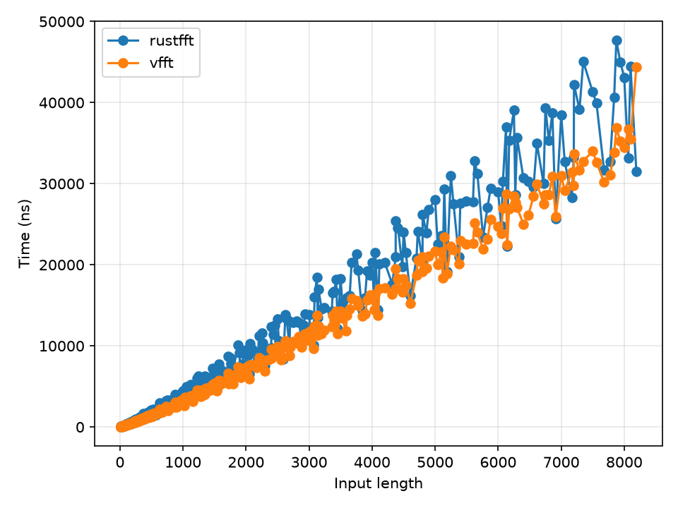
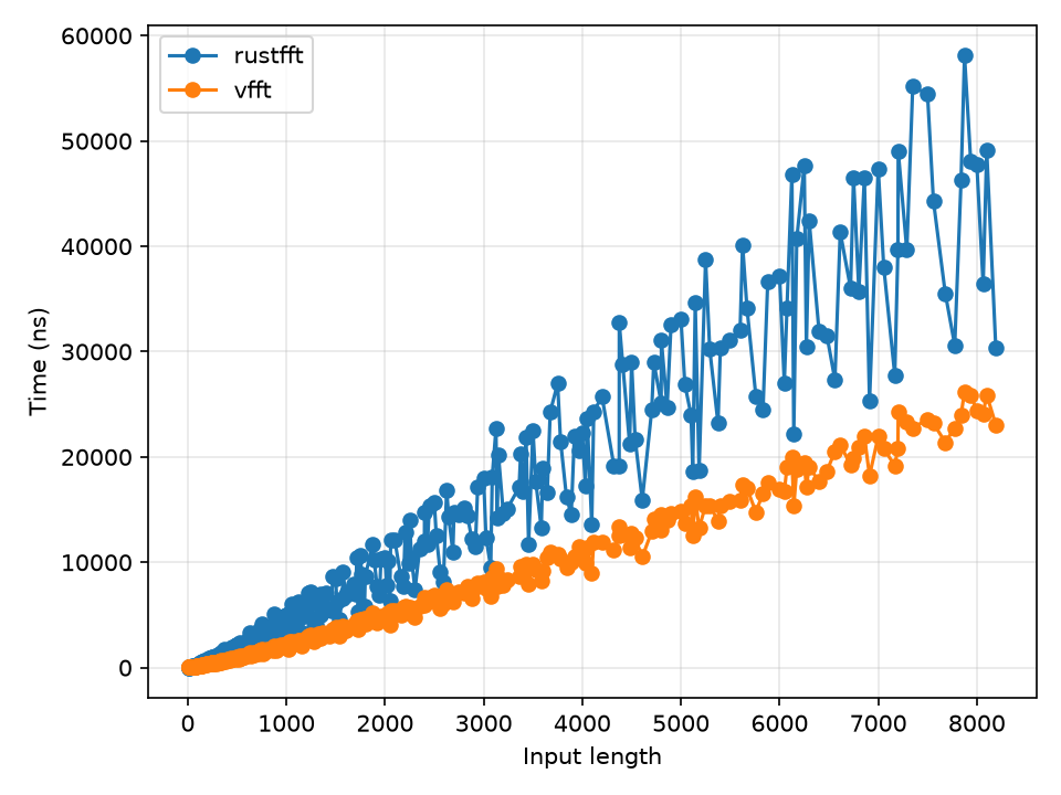
For whatever reason, Apple’s M5 chip adores my FFT, while my 9800x3d is merely pleased.
Here’s another view, showing the ratio of the vfft runtime divided by the rustfft runtime at the same input size. Anything below 1 means we’re beating rustfft:
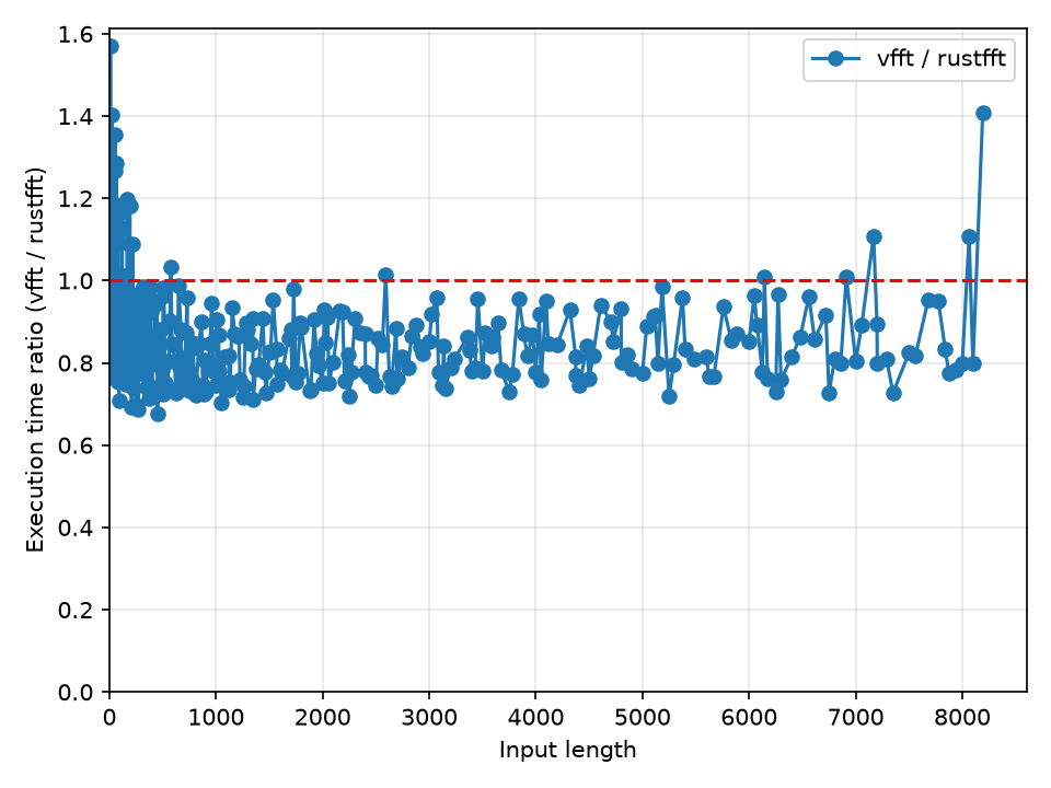
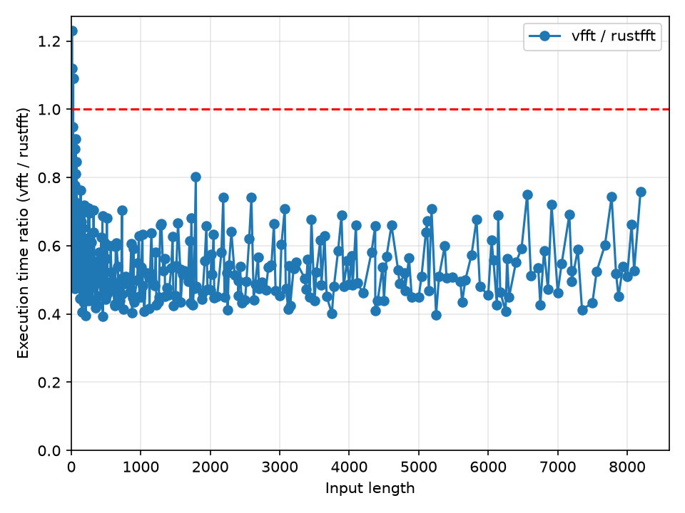
The 9800x3D wins in 91.2% of trials, where the M5 wins in 99.0% of trials, and by a much wider margin.
With these changes, vfft can now handle 307 input sizes between 9 and 8191, up from 10 before. It makes the tool far more flexible, which will be extremely useful in my ocean wave simulation. It achieves this without regressing on the power-of-two input sizes at all.
Note that we are still only measuring scalar performance. I have not touched SIMD at all yet, so we haven’t taken on the absolute best that rustfft has to offer. More on that later ;-)
All source code is available here. Check out commit
c4286017d3e88d2e and look at src/cpu.rs. Run tests with
cargo test -- --no-capture and benchmarks with
cargo bench. (The benchmarks take ~1.5 hours to run in
full. Edit benches/meow.rs if you want to test fewer sizes.)
I used AI to check my code for errors and investigate likely high-value optimizations. All committed code, and all prose / math in this article, was written entirely by me. I generated graphs with matplotlib (see plot.py in measurements/ in the repo), and made the diagrams with app.diagrams.net.